


We always want higher resolution when it comes to X-ray CT (Computed Tomography), micro-CT, or any imaging technique for that matter. The higher, the better, right? Well, not exactly. The tricky thing is that the resolution is usually in a trade-off relationship with something else that is also important, such as data collection time or SNR (signal-to-noise ratio). So the important question is not “How do we improve the resolution?” but “How do we optimize the resolution?” Also, to optimize it, we need to know what resolution is high enough for what we are trying to achieve.
What resolution is high enough?
Read: What is micro-CT?
What makes discussions about resolution confusing is that people might mean different things by “resolution.” This is not just for X-ray CT but for any analytical techniques. When people ask, “What is the resolution of [fill the blank]?,” you are not sure what exactly they are referring to. For X-ray CT, it can be the voxel size, detector pixel size, spatial resolution, sensitivity to different densities, or accuracy of dimensional analysis.
So in this article, I’m going to summarize different definitions of resolution and their implications to X-ray CT analysis, with a focus on the submicron to micro-CT range, then discuss how you can optimize the resolution in general by answering the following questions:
- What is resolution?
- What is the resolution limit of X-ray CT?
- Why isn’t higher resolution always better?
- How can we optimize resolution?
- How can we measure resolution?
- What about super-resolution?
1. What is resolution?
This is an important question. If we don’t know what it is, we can’t optimize it. So here you go: “Resolution is the ability of the measurement system to detect and faithfully indicate small changes in the characteristic of the measurement result.” according to NIST/SEMATECH e-Handbook of Statistical Methods. In other words, you see it if the resolution is high enough, and you don’t see it if the resolution is too low, whatever “it” is that you are trying to see. It sounds like a straightforward definition.
Then why is this subject so complicated? One reason is that people can be thinking about different things as “it.” As I mentioned at the beginning, “it” can be many things for CT. But we are going to define “it” as a very small feature we want to see for practical reasons. In this case, spatial resolution is the critical parameter. For example, if you’re going to see individual fibers in CFRP (carbon fiber reinforced polymer), the diameter of the carbon fiber (5 – 10 microns) is the smallest thing we need to see. The spatial resolution needs to be better than 5 – 10 microns to see these fibers. If you want to do quantitative analyses such as fiber orientation analysis, you need a lot better resolution, up to 1 micron or submicron spatial resolution. We will get into this in a bit.
Spatial resolution in radiography means the minimum resolvable separation between high-contrast objects. Note that the objects are assumed to have high contrast, and the noise level is sufficiently low. In digital imaging, the spatial resolution comes from two components: The pixel (or voxel) resolution and the point spread function (PSF). We will look into the latter in a moment, but for now, we can think of it as blurriness of the image.
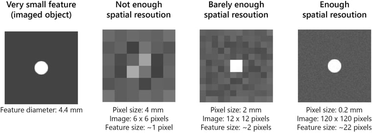
First, let’s compare different pixel resolutions in 2D images. This concept can be extended to 3D CT images by substituting “pixel” with “voxel.” The figure below compares 6 x 6, 12 x 12, and 120 x 120 pixels images of a 4.4 mm diameter feature. The 6 x 6 pixels image with 4 mm/pixel resolution has only one pixel to represent the feature. This is not enough to even detect the feature. The 12 x 12 pixels image with 2 mm/pixel resolution has only two pixels to represent the feature. This is enough to detect the feature but not enough to evaluate its size and shape quantitatively. The pixel size of the 120 x 120 pixels image is 0.2 mm/pixel and has 22 pixels to represent the feature. This is enough resolution to detect the feature and quantify its size.
This is a graphical representation of the relationship between the feature size, the spatial resolution, and the pixel resolution. And it tells us that the pixel size needs to be half or smaller than the feature size to see that it is there. In information theory, this rule is called the Nyquist-Shannon Sampling Theorem. The takeaway for X-ray CT is that the voxel resolution needs to be at least half or smaller than the feature size you hope to image.
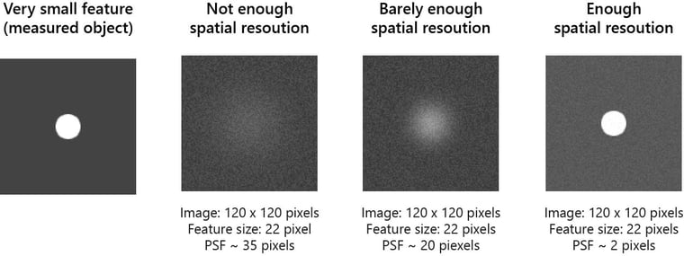
Let’s think about the PSF or the blurriness next. All images below are 120 x 120 pixels in size with 0.2 mm/pixel resolution. But, their blurriness is different due to the different PSF values. When the PSF is 35 pixels, greater than the feature size, the image is too blurry, and you cannot detect the feature. When the PSF is 20 pixels, roughly equal to the feature size, you can see that the feature is there, but the image is unclear. When the PSF is 2 pixels, about 1/10 of the feature size, you can clearly see the feature and its shape.
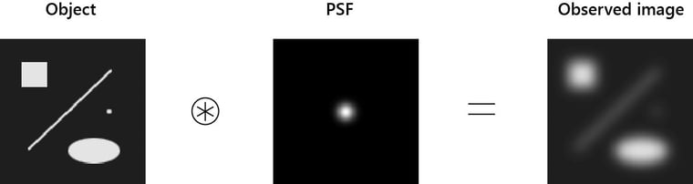
The PSF is a way to describe the response of an imaging system to a point source or point object. If we image a complex object through an imaging system, we will observe a convolution of the object and the PSF. The figure below is a graphical representation of how the PSF blurs the observed image.
Now we understand that the spatial resolution is defined by the pixel (or voxel) resolution and the PSF. The spatial resolution is also affected by the contrast, SNR, and artifacts, including the partial volume effect, but that is for another article. Now let’s connect these two main parameters to the components of an X-ray CT scanner, which we can control to optimize the resolution. The diagram below shows the elements affecting the spatial resolution.
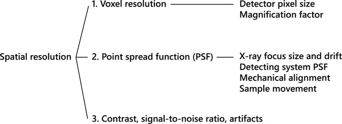
The voxel resolution is simply the size of the voxel of a CT image. It is defined as the detector pixel size divided by the magnification factor. You can artificially make the voxel smaller by chopping it up into pieces, but that does not increase the spatial resolution. The PSF is a bit more complicated. As illustrated in the figure below, it is affected by everything from the X-ray focus size and drift, the detector’s PSF, the scintillator’s PSF, and if you have a lens, the PSF of the lens system.
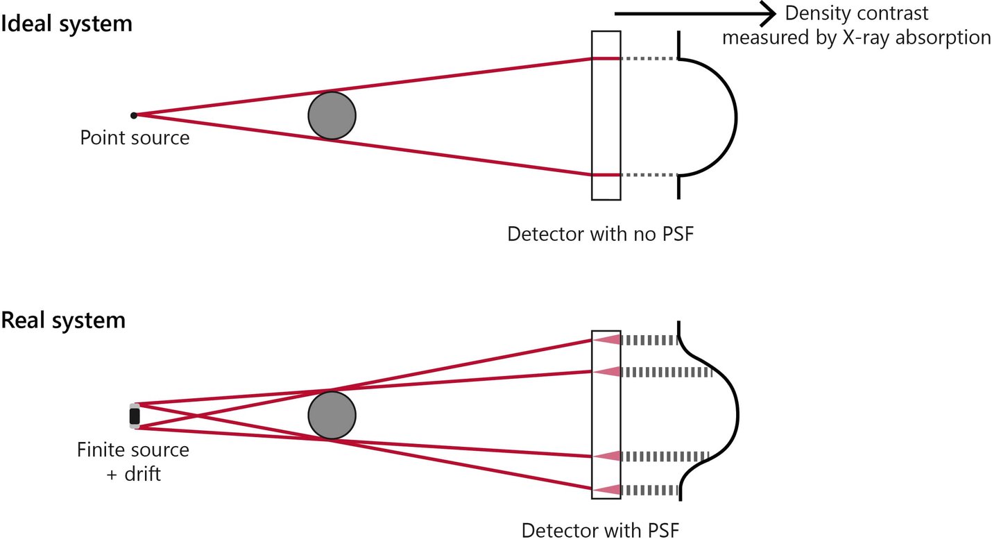
The mechanical alignment of the X-ray focus, scan rotation center, detector center, and the tilt of the detector all affect the PSF. The sphere of confusion (wobbling) of the scan rotation axis can increase the PSF. And lastly, if the sample moves or changes its shape during a scan, that also increases the PSF. Many of these factors are fixed by the CT scanner you use, but there is room for optimization. You can skip to sections 3 and 4 to see how to optimize the resolution. Or, you can take a moment to think about X-ray physics. How high can the resolution of X-ray imaging be, theoretically?
2. What is the resolution limit of X-ray CT?
The spatial resolution of X-ray CT depends on the CT scanner. It varies from several tens of nanometers to sub-millimeters. Medical CT scanners and large-scale industrial CT scanners are on the sub-millimeter side of the spectrum. Micro-CT scanners are in the few to hundreds of microns range. High-resolution CT scanners equipped with optical lenses can achieve submicron resolution. Then by adding Fresnel zone plates or multilayer optics, you can achieve 10-50 nm resolution. If you are a microscopist, you might ask, “Why is it limited only to 10 nm when X-ray wavelength is a lot shorter than that?” That is an excellent question.
The principal limit to the resolution of any optical device is somewhere around the wavelength of the light used in the imaging experiment. Light with wavelength λ, traveling in a medium with refractive index n and converging to a spot with half-angle θ has a minimum resolvable distance of d = λ/(2n sinθ) = λ/2NA. N is the numerical aperture.
For optical microscopy, this means the resolution limit is at the sub-wavelength level. However, the numerical aperture is extremely small for X-rays because the refractive index is almost 1 for most media, and we can’t make lenses easily. So, for example, the wavelength of X-rays at 10 keV is 0.124 nm, but the practically achievable resolution is more like 10 – 100 nm even when synchrotron radiation and mirrors (100 nm, Matsuyama et al., 2016, Sci. Rep., 6:24801) or Fresnel zone plates (10 nm, De Andrade et al., 2021, Adv. Mater., 33(21), 2008653) are used. With the laboratory-based CT scanners, the X-ray focus size and detector PSF are often at micron-level, keeping the practical resolution in the submicron to submillimeter range.
3. Why isn’t higher resolution always better?
Higher resolution is not always better because the resolution is usually in a trade-off relationship with the FOV (field of view), data collection time, and SNR. Let’s take a look at each parameter.
Resolution vs FOV
At a fixed magnification setting, the FOV is defined by the size of the detector, as shown in the figure below. A flat panel, CCD, or sCMOS are commonly used as the detector. All detectors have a limited number of pixels, generally ranging from 1000 x 1000 to 3000 x 3000. This means that the voxel size is limited to 1/1000 ~ 1/3000 of the FOV size. This is a limitation coming from today’s X-ray detector technology. Increasing the resolution, that is, decreasing the voxel size, reduces the FOV size. So higher resolution might mean sacrificing the FOV.
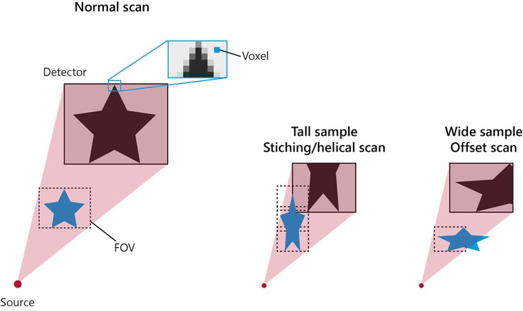
There are a few workarounds, though. If the sample is tall, you can use vertical stitching or a helical scan to increase the resolution without sacrificing the FOV size. If the sample is wide, you can use an offset scan to increase the resolution while keeping the FOV twice the detector width. When using these techniques to widen the FOV while increasing the resolution, pay attention to the file size. A high-resolution and large FOV scan can result in a very large file that you might not be able to open and analyze later. The file size can be calculated with the following equation:
P1 x P2 x P3 x bit depth [bits] = P1 x P2 x P3 x bit depth / 8 [bytes]
P1, P2, and P3 are the number of pixels in X, Y, and Z directions. The bit is the gray level bit depth, normally 8 or 16. For 1000 pixel cube with 16-bit depth is 2GB, for example. Depending on the analysis software and computer you use, 2 – 20 GB files are manageable.
Resolution vs data collection time and SNR
Next, let’s think about the data collection time and SNR. The number of X-ray photons is generally limited by the X-ray source we use. So, if we increase the resolution by changing the magnification factor, the solid angle of X-rays the detector covers decreases. As a result, the total number of X-ray photons counted by the detector decreases.
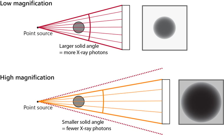
Low X-ray count causes low SNR and makes the resulting CT image noisy. You can improve SNR by increasing the scan time.
We can also decrease the X-ray focus size, that is to decrease the PSF, to increase the resolution. To decrease the focus size on commonly used micro-focus X-ray tubes, we need to decrease the filament current. This also reduces the X-ray count and decreases the SNR.
If you are combining multiple pixels (binning) to generate one voxel during the reconstruction calculation, you can decrease the voxel size down to the size of one pixel to increase the resolution. But this again means that the number of X-ray photons that contribute to one voxel reduces, and the SNR decreases.
Either way, you can see that increasing the resolution reduces SNR or increases the measurement time. So you want to optimize the resolution depending on the power of the X-ray source and the time you have.
4. How can we optimize the resolution?
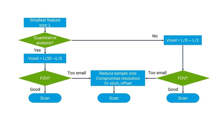
With everything we reviewed up to this point in mind, let’s figure out how to optimize the resolution. As we discussed at the beginning of this article, the size of the smallest feature we need to see is the determining factor. So start by defining it. Let’s say that size is “L.” If it is enough just to identify that feature is there, set the voxel size to L/5 ~ L/2. If you plan to quantify the shape, size, etc., of that feature, then set the voxel size to L/20 ~ L/5.
Remember that the higher the resolution is, the longer the scan takes to achieve the same data quality. The voxel size should define the FOV and magnification factor on a given CT scanner. If the FOV is the size you want, normally close to your sample size, you are ready to set up a scan. If the FOV is too small, you can either reduce the sample size, compromise the resolution, or use FOV enhancement techniques such as stitching or an offset scan.
The X-ray energy should be optimized based on the sample density and size. The number of projections, scan time, etc., should be optimized based on the SNR you need to achieve and how much time you have.
Read: How to Improve the Signal-to-noise Ratio of X-ray CT Images
5. How can we measure resolution?
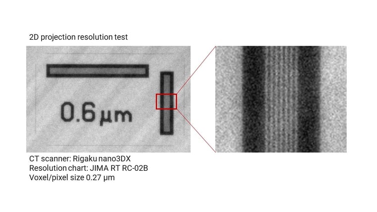
Now, how can we test the resolution? As we saw at the beginning of this article, the resolution of X-ray CT images is not defined just by the voxel size. Even if the voxel size is 1 micron, many components of a CT scanner can blur the image, and you might not be able to even see even features of 5 microns in size. So how can we know the real resolution of a CT scan? The best way to do that is to measure it using a resolution standard. Resolution standards have line pairs of high and low absorption materials, silicon and polymer, for example. Some resolution standards are made for a 3D scan and are called resolution phantoms. Others are meant for a 2D projection. Below is an example of a submicron resolution test.
Here are some of the commonly used resolution standards:
- QRM Micro-CT BarPattern (3D phantom for 5 – 150 microns)
- QRM Micro-CT BarPattern Nano (3D phantom for 1 – 10 microns)
- JIMA RT RC-02B (2D chart for 0.1 – 15 microns)
6. What about super-resolution?
Super-resolution is a general term for techniques used to upscale (increase the resolution of) images. For X-ray CT, the term usually refers to a technique that improves the resolution using deep learning. (See a survey by Park et al., 2018, Phys. Med. Biol. 16;63(14):145011 or watch a Dragonfly webinar on super-resolution.) This technique has been intensively studied for medical applications as a way to reduce radiation dosage without compromising the image quality. Applications to materials science have been published in recent years. (See an application example for rock analysis application by Wang et al., 2019, J. Pet. Sci. Eng., 182, 106261.) Most deep learning super-resolution techniques require training data, but there are a few that do not. It is an artificial way of increasing resolution and should be used with caution. But it can be very useful for 4D CT experiments where a good training dataset can be available and the scan time needs to be extremely short.
Takeaways
So the takeaways are: Higher resolution is not always better. What is important is to know the resolution you need and figure out the best way to achieve it, and understand what might be compromised along the way. Also, don’t simply take the voxel resolution as the resolution. Consider other factors that can blur the image. When in doubt, it is always best to measure the resolution. I hope you are ready to get back to the lab and tweak scan conditions to improve the quality of your CT images. If you have any suggestions or questions, please let us know. Our team of application scientists can help you figure out how to optimize the measurement conditions for your specific imaging needs. You can talk to one of our CT experts by clicking the “Talk to an expert” button at the right top of the page or send us a message at imaging@rigaku.com.