What Is Beam Hardening in CT?

You just scanned your sample and are running reconstruction, waiting for the CT image to come up, excited to see what you will find. Then you get weird shadowing like this, although the material density should be uniform: 

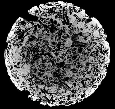
 (⅓-inch diameter carbonate plug scanned at 130 kV with 1 mm Al filter) 

Then you start having nightmares about the painful segmentation process you have to deal with, or you might even—regretfully—give up on analyzing these samples. 

Does this sound familiar? If it does, you came to the right place. You have a beam hardening problem, and I can help you with that. 

Beam hardening is notorious for causing nasty artifacts in CT (computed tomography) images. These artifacts are problems not only with micro CT used for industrial inspection and materials research but also with medical CT. 

I hated and complained about beam hardening over the years. While figuring out what to do with it, I also learned why it happens and how to deal with it better. 

If you suffer from beam hardening artifacts and want to get rid of them, you are not alone. While you usually can’t completely remove them, there are ways to handle them. However, we must first understand what the sources of the problem are to handle it better. So, to help you with all your beam hardening problems, I will address the following questions in this article: 

What is beam hardening? 

What causes beam hardening? 

What causes beam hardening artifacts? 

Why is beam hardening important? 

How can I reduce beam hardening artifacts? 

Download PDF

What is beam hardening? 

The energy distribution of X-rays shifts toward the higher side as X-rays go through an object. This phenomenon is called beam hardening.  

High-energy X-rays are also known as “hard” X-rays, which can penetrate denser, thicker materials better than low-energy X-rays or “soft” X-rays. In other words, X-rays harden as they penetrate an object. Hence the name, beam hardening. 

For example, we generate X-rays using an X-ray source with a tungsten target and a 150 kV excitation voltage. The generated X-ray energy distribution looks like the graph below on the left. (Note that this is a general representation of the X-ray spectrum, and the shape of this graph can change slightly depending on the X-ray take-off angle, X-ray window material and thickness, etc.) 

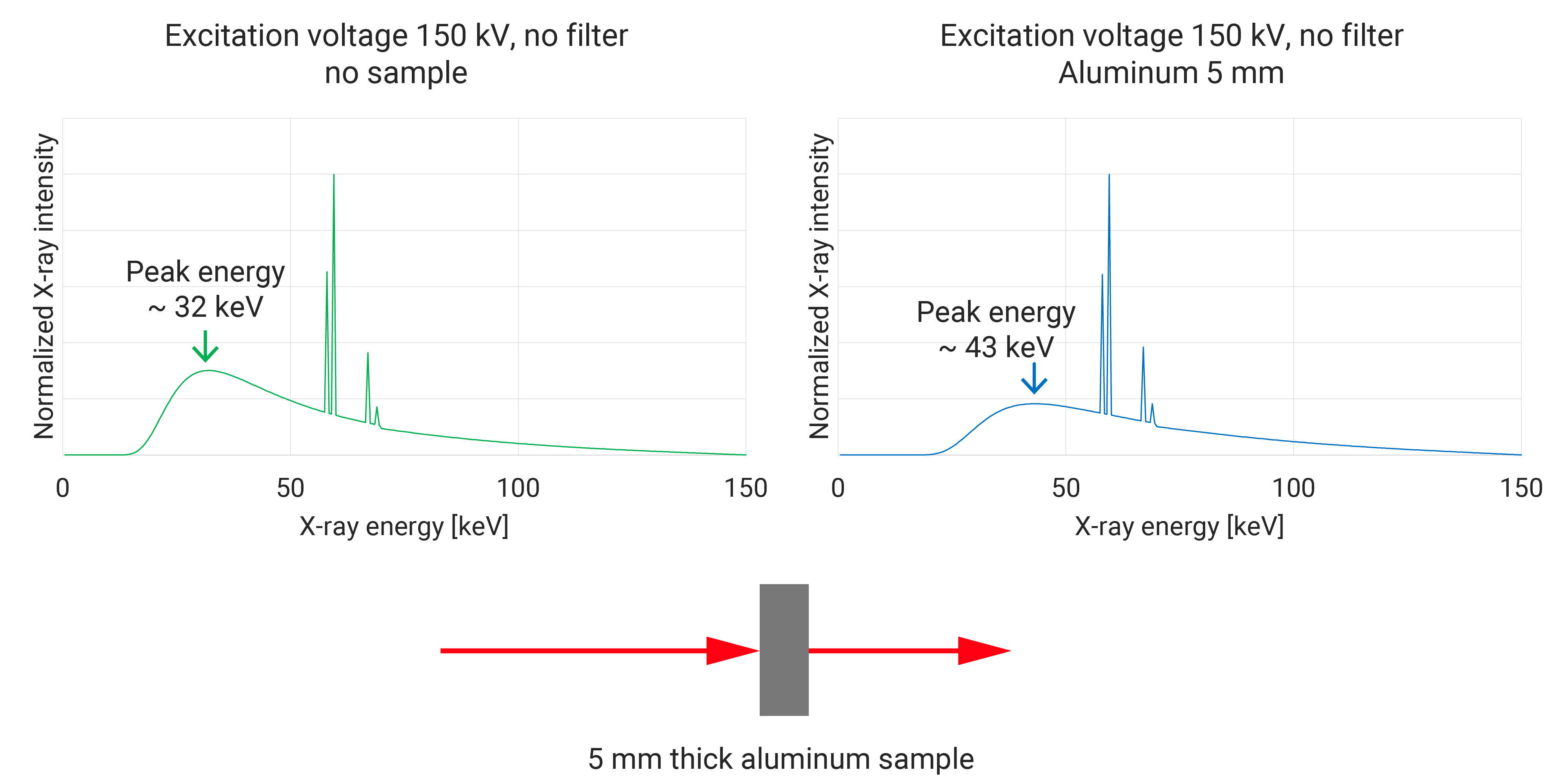
The peak of the bremsstrahlung X-rays—the broad and continuous spectrum—is about 32 keV before X-rays go into the sample. This peak shifts after going through a sample, as we will see in a second. The sharp peaks are tungsten’s characteristic radiations, and their energy shift after going through a sample is negligible. This means monochromatic X-rays don’t harden. 

Now let’s look at the energy distribution after the X-rays go through a 5 mm thick aluminum plate, the graph above on the right. The bremsstrahlung X-ray spectrum shifted towards the higher side, and the peak energy changed from 32 keV to 43 keV. The X-rays hardened after going through the aluminum plate. (Note that normalized intensities are shown.) 

This energy shift causes beam hardening artifacts and is often considered a problem, but there is also a benefit. When you need to increase the X-ray energy, but the available excitation energy is limited, you can add a filter to intentionally cause beam hardening and increase the X-ray peak energy (pre-harden the X-rays), as you can see in the calculation below. 

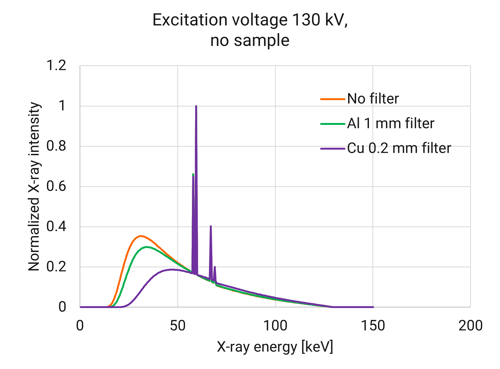
In this example, the excitation voltage was kept at 130 kV and the spectrum was calculated for different filter materials and thicknesses. You can see the bremsstrahlung radiation peak shifts depending on the filter, while the characteristic radiations (sharp peaks) don’t. 

Now, why does the energy distribution shift? In other words, what causes X-rays to harden? 

What causes beam hardening? 

Before getting into the cause of beam hardening, let’s review the types of X-rays. 

We can categorize X-rays into two types based on their energy distribution: monochromatic and polychromatic. The former has no or minimal energy width, as in characteristic radiation, while the latter has a broad energy distribution, tens to hundreds of keV, as in bremsstrahlung radiation. 

Characteristic radiation is monochromatic and often used as a probe in X-ray diffraction analysis or as a signal in X-ray fluorescence analysis. Synchrotron radiation is also usually monochromatic after going through a monochromator to select a narrow energy range. 

Let’s think about the X-ray absorption process with monochromatic X-rays first, because this is how most of us envision X-ray absorption. 

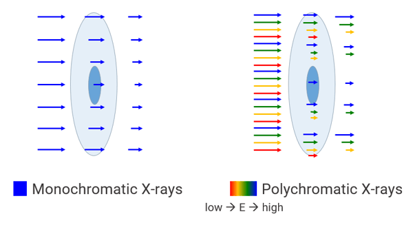
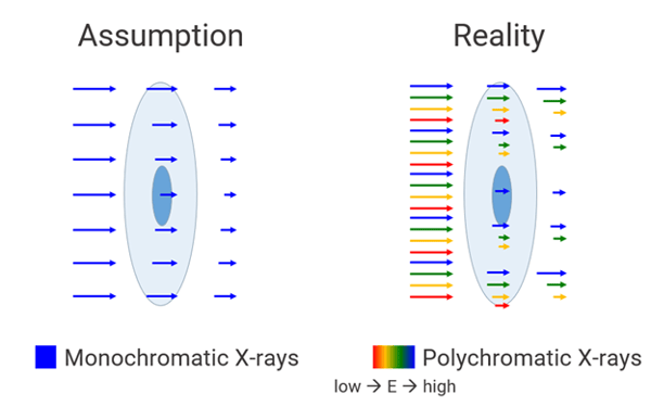
Suppose monochromatic radiation travels through an object of varying thickness and density, represented by blue arrows on the left side of the diagram below. The color blue represents the single X-ray energy; the lengths of the arrows represent the X-ray intensity. 

The incident X-rays have uniform intensity distribution. As they travel through the sample, the intensity of the X-rays going through thin and low-density regions of the object (top and bottom) decreases only a small amount. 

Meanwhile, the intensity of the X-rays going through the thick and high-density areas of the object (middle) decreases substantially because the thicker and denser the object, the more X-rays are absorbed. 

In this case, the spatial distribution of X-ray intensity changes, giving us a radiograph of the object, but the X-ray spectrum remains the same. Thus, no beam hardening occurs. 

Let’s think about polychromatic X-rays next. 

Suppose polychromatic radiation travels through an object of varying thickness and density, as shown on the right side of the diagram above. The color and length of the arrows represent different energies and X-ray intensities, respectively. 

To keep it simple, let’s assume the incident X-rays have uniform intensity distribution over a range of energy and space. Then, as they travel through the sample, the intensity of the X-rays going through thin and low-density regions of the object (top and bottom) decreases only a small amount. 

Meanwhile, the intensity of the X-rays going through the thick and high-density areas of the object (middle) decreases significantly. This much is the same as the case of monochromatic X-rays. 

However, you can see that the blue (high-energy) X-rays are absorbed less than the red and yellow (low-energy) X-rays. This is because the blue (high-energy) X-rays have a lower absorption rate—they are harder in other words—than the red and yellow (low-energy) X-rays for the same material. 

Because of this difference in absorption rates, we have more blue (high-energy) X-rays and fewer red and yellow (low-energy) X-rays after the object absorbs X-rays. This means X-rays were hardened in this process. 

To summarize, the broad energy distribution and the energy-dependent absorption rates of an object cause beam hardening. Beam hardening is negligible when the object’s absorption rate doesn’t vary much within the X-ray energy distribution or when monochromatic X-rays are used. 

Now, why is this such a problem? 

What causes beam hardening artifacts? 

Most reconstruction algorithms assume monochromatic X-rays mainly for two reasons: 

1. We can’t fully calculate the beam hardening effects polychromatic X-rays experience without knowing the absorption rate mapping inside the sample. 

1. Even if we knew the absorption rate mapping inside the sample, it would be too computationally taxing to consider the energy distribution of polychromatic X-rays. 

In reality, assuming monochromatic X-rays in the calculation while using polychromatic X-rays creates a mismatch between the calculation and the reality of the X-ray absorption process. 

This mismatch causes artifacts. The most common beam hardening artifact is varying gray level within a uniform density object. The area close to the surface of a bulky sample tends to have a higher value (lighter gray) than the center area, as we saw in the example at the beginning. 

Now, we can see that ignoring the energy distribution of polychromatic X-rays can cause errors in the reconstructed gray levels, but why does this make the edge brighter than the center of a bulky object? 

On the left of the diagram below, you see a top view of a cylinder-shaped sample, like a drill core or a plug, in the cone beam geometry setting. On the right, you see CT cross-sections with and without beam hardening artifacts. 

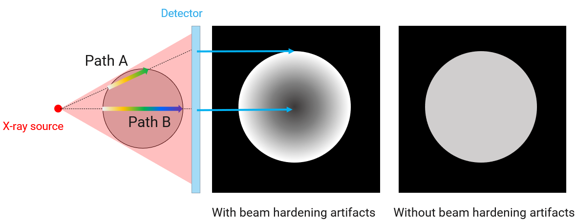
Let’s consider what happens to the polychromatic X-rays that go through path A and path B, which contribute to the outer edge and center of the reconstructed cross-section shown on the right. 

The difference in the path length is, wrongly, translated into a difference in density because of beam hardening. That is why the outer edge appears brighter than the center in a bulky sample, even when the material density is constant. 

Here is another example of a bulky sample with a uniform density. It has a more complex shape: 

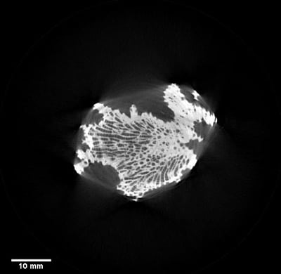
The figure above is a cross-section of a coral reef collected at 90 kV with a 1 mm thick aluminum filter. In this example, the gray level is uneven inside the coral reef, with the near-surface area appearing brighter than the center area. In addition, there are gray streaks around the sample where it should have a uniformly dark background, representing air. 

In this example, the sample contains only one material, calcite. When the sample contains both low- and high-density materials—plastic and metal, for example—more complex beam hardening artifacts can occur. 

When some parts of the sample are extremely dense and thick compared to the matrix, almost no X-rays can get through the dense parts. In this case, we can’t get enough information from the X-ray projection images. This phenomenon is different from beam hardening and is called photon starvation. It causes severe artifacts. 

Here are examples of the main artifacts caused by high-density materials in a sample: 

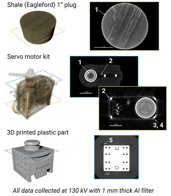
We see multiple types of artifacts in this figure. Sometimes, they are all grouped together and referred to as beam hardening artifacts. However, some of them are caused by different X-ray absorption and scattering phenomena. 

1. Varying gray level of a uniform material - caused by beam hardening (other names: shading or cupping artifacts) 
2. Dark streaks extending from bright (high-density) objects - caused by photon starvation (another name: metal artifacts) 
3. Saturation of the gray level around bright (high-density) objects - caused by the wide range of densities in the sample (another name: metal artifacts) 
4. Halo of the lighter gray level around bright (high-density) objects - caused by the X-ray scattering (another name: metal artifacts) 
5. Dark streaks extending from flat surfaces - caused by the refraction of the X-rays 

Why is beam hardening important? 

Now we understand what beam hardening is and what causes it. Why is this important? 

X-ray CT analysis often aims to quantify the sample's characteristics, such as void distribution or part dimensions. To quantify these parameters, we need to segment the image into different phases or identify the location of the surface. Beam hardening artifacts, along with other artifacts, make this segmentation or surface identification process difficult or inaccurate. 

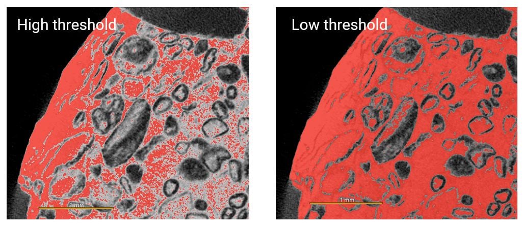
Let’s see what happens if we try to segment the first image of a carbonate plug we saw at the beginning. If we set the threshold high to leave the voids close to the surface unselected, the solid part near the center is also not selected because it is darker than the edge due to the beam hardening artifacts, as shown on the left in the figure below. 

Decreasing the threshold to select the center area, in turn, causes the voids near the surface to be identified as solid. So, we cannot use thresholding to segment this image. This is the typical problem of beam hardening, and it is crucial to understand why beam hardening occurs and how to deal with it to generate accurate segmentation. 

How can I reduce beam hardening artifacts? 

There are several ways to deal with beam hardening. The common approach is to reduce them, either by changing data collection parameters or by implementing a beam hardening correction in the reconstruction process. 

Here are several approaches: 

1. Increase the X-ray energy by increasing the excitation voltage 

This approach has virtually no side effects except for the fact that you lose contrast in the low-density area if the sample is a mixture of high- and low-density materials. 

This approach has the same side effect as increasing the excitation voltage. In addition, a denser and thicker filter reduces the X-ray intensity and increases data collection time. 

This approach is less common because it requires a special X-ray source with characteristic or synchrotron radiation, which might not be readily available. 

This approach’s side effect is that you might have to cut the sample and work with a smaller field of view. 

This approach doesn’t have side effects, but it doesn’t necessarily work for all cases, depending on how the correction is applied. 

        Read: How to Reduce Beam Hardening Artifacts in CT

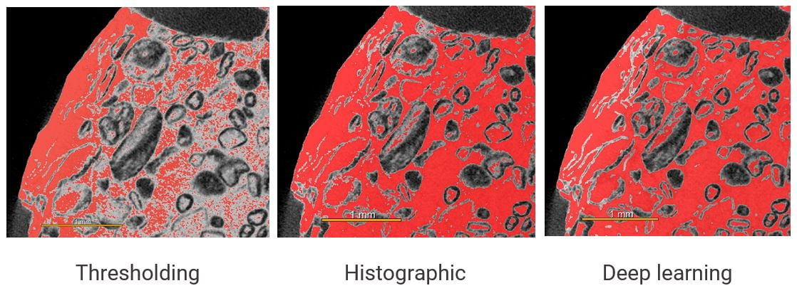
These are ways to reduce beam hardening artifacts. However, there is a different way to look at this problem. The problem is not the beam hardening artifacts themselves but the difficulty they cause in image segmentation. When we look at it this way, we don’t need to change the data collection or reconstruction strategy. Instead, we change how we segment the image. 

As we saw previously, we couldn’t segment the CT image of the carbonate plug using gray-level thresholding. We can use more sophisticated segmentation algorithms such as histographic and deep learning segmentation. As you can see in the example below, these techniques provide correct segmentation despite the uneven gray level caused by beam hardening. 

What should I do now? 

Have you given up on analyzing some samples with beam hardening artifacts? Or are you spending a lot of time manually segmenting a CT image with beam hardening artifacts? If so, I hope this article will help you understand why your sample exhibits beam hardening artifacts and try to reduce it to get more accurate analysis results faster. 

Take a look at examples of beam hardening reduction and see which one works best for your sample. 

If you are not sure where to start, our team of CT experts can look at your CT images and help you figure out the best way to improve the image quality. You can talk to one of our CT experts by clicking the “Talk to an expert” button at the right top of the page or send us a message at imaging@rigaku.com.