


When you run a CT (computed tomography) scan, you always run a reconstruction calculation to convert the 2D projections to 3D volume data. Have you ever wondered how reconstruction works?
Why can we see cross-sections of an object without sectioning it? What happens when the 2D radiographs or projections go into a reconstruction program and come out as 3D volume CT data?
If you have been pretending to understand how reconstruction worked and can’t answer these questions, you are not alone. Many CT users give up on understanding this essential part of the CT technique. That is okay because you can still use CT and benefit from it without understanding how exactly CT images are created.
However, you might be curious and want to know how it works. If that’s the case, I hope this article will help you. I will show you how reconstruction works and explain terms you’ve heard but never understood, such as Radon transformation and sinograms.
How does filtered back projection work?
I’ve run the demonstration calculations using the open-source image processing program ImageJ. If you want hands-on experience and to deepen your understanding of reconstruction, watch this on-demand workshop and follow the exercises.
What is CT reconstruction?
When we run a CT scan, we collect radiographs or 2D projections. All portions of the sample in the X-ray beam path get projected on top of each other. How do we convert them into a 3D map of the object or a collection of tomographic cross-sections? This process of restoring the original higher-order dimensions from lower-order observable values is called reconstruction.
Reconstruction is arguably the most important concept in X-ray CT. Because most artifacts are generated in this process, it is vital to understand reconstruction to prevent or reduce them. However, reconstruction is also the most confusing part of image processing involved in CT.
Reconstruction or 3D rendering?
Some people are confused about which part of their everyday data processing is reconstruction. Displaying a 3D rendering of a sample is not a reconstruction process. Reconstruction happens before you get to that point.
During data collection, we collect 2D projections observed on the detector. (Note: These can be 1D profiles when a line detector is used.) Then we convert the 2D projections into 3D data or a set of CT cross-sections. This is the reconstruction process. The result is what you recognize as a TIFF stack or a DICOM file consisting of hundreds to thousands of CT cross-sections.
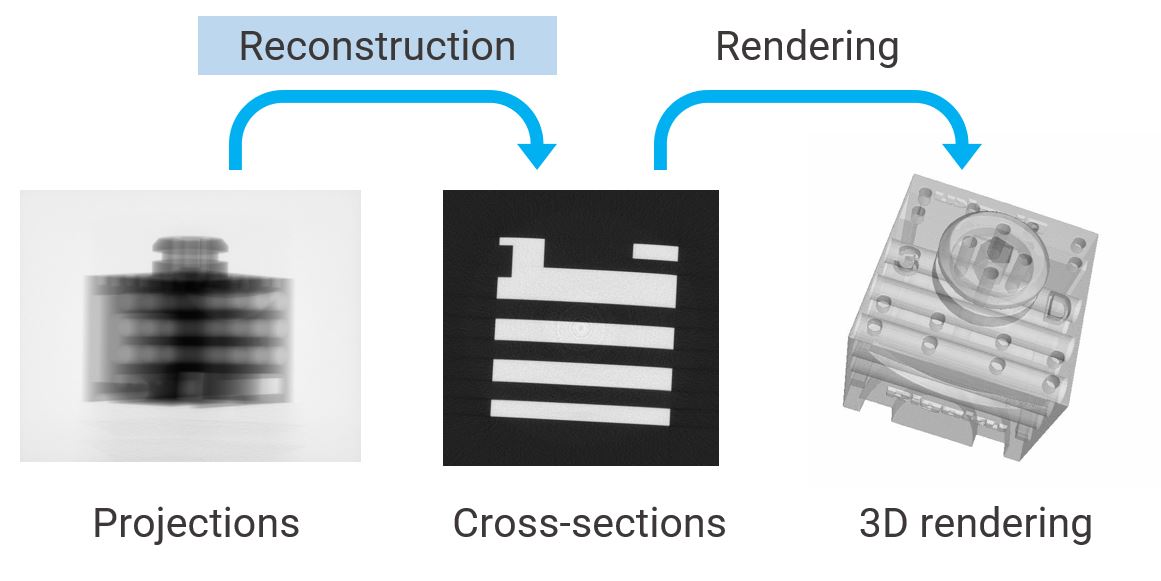
Different stages and representations of X-ray image data: projections, cross-sections, and 3D rendering (an example of a 3D printed plastic object)
As you see in the figure above, we sometimes see a CT scan represented as a 3D-rendered view. This is merely a representation of already reconstructed CT data.
X-ray CT Geometries
As we will see later, reconstruction is an attempt to “back-calculate” the absorption coefficient distribution in the sample based on the observed projections. To do this, we need to model the X-ray CT geometry.
The figure below shows three commonly used X-ray CT geometries. To keep it simple, we will focus on parallel beam geometry in this article. You can extend the theory we will review here to other geometries.
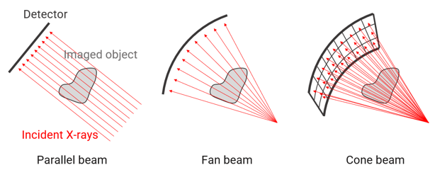
If you are interested, this video shows how the filtered back projection calculation is extended from parallel beam to fan beam geometry: Intro to Digital Image Processing by Rich Radke - # 19 Fan beam reconstruction.
I highly recommend this intro course by Dr. Radke if you are interested in learning the nuts and bolts of image processing.
Who invented reconstruction?
Johann Radon first presented the concept of reconstruction in 1917. The word “tomography” didn’t even exist then, but his theory proved that CT reconstruction was possible. If interested, you can read the original paper: Radon, J. On the determination of functions from their integral values along certain manifolds, IEEE Trans. Med. Imaging, 5 (4). (English translation published in 1986)
It was later demonstrated by experiments, and commercial medical CT scanners became available in 1971. Sir Godfrey N. Hounsfield and Allan M. Cormack were awarded the Nobel Prize in Physiology or Medicine in 1979 for developing commercial CT scanners.
A variety of reconstruction algorithms
More than a century has passed since Johann Radon came up with the concept of reconstruction. Today, there are a variety of reconstruction algorithms.
Here is a non-exhaustive list:
- Algebraic Reconstruction
- Iterative Reconstruction
- Filtered Back Projection
- Convolution Back Projection
- Deep Learning Reconstruction
We will review the most commonly used algorithm, the Filtered Back Projection, later. First, let’s review the algebraic reconstruction technique (ART), because it is the most basic concept and helps us see that reconstruction is possible.
Algebraic Reconstruction Technique
This technique, as its name indicates, algebraically reconstructs the original absorption coefficient distribution.
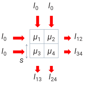
To keep it simple, we consider a 2-by-2-pixel object. The pixel thickness is s, and each pixel has a unique linear absorption coefficient µ1, µ2, µ3, and µ4 as shown in the figure below. We put an X-ray beam with intensity I0 through the sample in the horizontal direction and observe the transmitted X-ray intensities I12 and I34.
Then we change the X-ray beam direction and repeat the same experiment in the vertical direction to obtain I13 and I24, just like we run a CT scan.
The relationship between the transmitted and incident X-ray intensities follows the Beer-Lambert law:
![]()
Where µ and s are the linear absorption coefficient and thickness of the object I0 goes through, respectively.
Using this relationship, we can describe the 2-by-2-pixel experiment as follows:
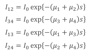
Here, we have four equations and four unknown parameters to determine the exact absorption coefficient distribution inside this 2-by-2-pixel object. Therefore, we can solve these relational equations to obtain µ1, µ2, µ3, and µ4.
This is how ART works. Because this is a direct calculation of the absorption coefficient distribution, it suffers from fewer artifacts than other techniques. It also tolerates a lack of projections better than other techniques. For these reasons, it is sometimes used for medical CT reconstruction. The downside of ART is that the calculation becomes slow when the field of view (FOV) becomes larger.
In the following sections, we will review key concepts involved in reconstruction to cover the bases, then look into how the Filtered Back Projection works.
What is a projection?
We have been using the term “projection.” Before discussing the Filtered Back Projection (FBP), let’s define what projection data is. This is an important concept to understand FBP.
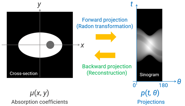
A projection is what we observe on the detector after X-rays transmit through an object. Let’s think of an experimental setup shown below. The scanned object is µ(x, y) and generates a projection p(t, θ) at angle θ at location t on the detector when X-rays I0 travel through it.
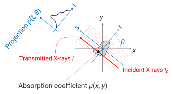
The transmitted X-ray intensity I follows Beer-Lambert law:
![]()
The linear absorption coefficient µ is a function of the location (x, y). This equation can be rewritten as follows:

Using this equation, we can define the projection p(t, θ) as absorption integrated through the thickness:

(equation *1)
You can see that a projection provides integration of the absorption coefficient along the object axis s as a function of projection angle θ at location t on the detector. This indicates we can use multiple projections to figure out the absorption coefficient distribution in the scanned object.
What is Radon Transformation?
You might have heard the term Radon transformation mentioned when discussing CT reconstruction. Wikipedia describes it this way: “In mathematics, the Radon transform is the integral transform which takes a function f defined on the plane to a function Rf defined on the (two-dimensional) space of lines in the plane, whose value at a particular line is equal to the line integral of the function over that line.”
While it is an accurate description of what Radon presented in 1917, proving that CT reconstruction is possible, it doesn’t help us understand its role in reconstruction. So, we will continue the discussion around projection data.
When we run a CT scan, we collect a set of projections p(t, θ) for a wide range of θ, typically 0 – 180° for parallel beam geometry and 0 – 360° for cone beam geometry. As we collect the data, we convert µ(x, y) into p(t, θ).
This conversion, expressed in equation *1, is the Radon transformation, also called the forward projection. In other words, the Radon transformation converts absorption coefficient distribution (the answer of CT reconstruction) to projection data (the observable of CT measurement).
What is a sinogram?
Another term you might have heard of is sinogram. It is not a medical test of the sinus in this context. In CT, a sinogram is a way to visualize projections in (t, θ) space. You might see sinograms in publications about reconstruction algorithms. They help us understand the relationship between the projection and CT data.
Let’s take a look at an example below. The figure on the left is a cross-section of an object. The gray level represents the absorption coefficients. You see a high-density (bright) egg-shaped object in the air (black). The “egg” has a low-density (gray) yolk-like circle. The absorption coefficient of each location is µ(x, y).
You can convert this cross-section µ(x, y) into p(t, θ) using equation *1. By plotting p(t, θ) in (t, θ) space, you obtain the sinogram, as shown on the right.
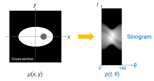
A sinogram has the X-ray angle θ and the detector position t as its axes. Let’s see what happens if we track a point in the cross-section as we run a CT scan.
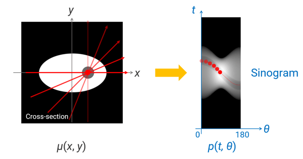
Let’s focus on the red spot in the middle of the gray “yolk,” as shown on the right in the figure below. When an X-ray beam goes through this spot from different angles from 0 to 90°, the projection corresponding to this red spot moves through the sinogram, as shown on the right. Its path follows a sine curve. This is where the term “sinogram” came from.
Why is this important? Sinograms are convenient representations of projection data, and they help us to better understand what is happening in projection space. For example, if something goes wrong during CT data collection or a detector has dead pixels, it is easier to spot them in a sinogram than the conventional representation of projections or reconstructed CT cross-sections.
The figure below shows examples of sinograms:
- A normal sinogram shows a collection of smooth sine curves.
- Vertical lines that are darker or lighter than the surrounding areas indicate that the entire detector or the X-ray source went dark or bright during the scan.
- An overall shift of the projection indicates the sample moved during the scan. When using parallel beam geometry, the projection at 180° should be a perfect mirror image of the one at 0°. In this example. The top and bottom edges shifted to the lower side at 180°, indicating sample movement.
- Horizontal lines that are darker or lighter than the surrounding areas indicate that the detector has hot, cold, or dead pixels that respond differently from the surrounding pixels.
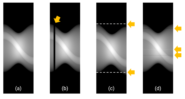
These abnormalities shown in (b), (c), and (d) cause various artifacts in the reconstructed CT images. Watch the on-demand workshop and follow the exercises to see what kind of artifacts show up for each case.
How does filtered back projection work?
As we reviewed earlier, the Algebraic Reconstruction Technique reduces artifacts and requires a relatively small number of projections. However, the calculation becomes complicated and takes a long time as the image matrix becomes large, a 3000 x 3000 x 3000 voxels cube, for example, a typical size of a micro-CT scan.
This is where the Filtered Back Projection (FBP) technique comes in handy. As the name suggests, it generates µ(x, y) by back-projecting p(t, θ).
In CT data collection, we observe projections p(t, θ) generated from the forward projection or the Radon transformation of µ(x, y). In the reconstruction process, we calculate absorption coefficient distribution µ(x, y) by back-projecting the observed p(t, θ).
The FBP calculates the back projection of p(t, θ) to reconstruct µ(x, y). Because we already know the forward projection follows equation *1, we can calculate the back projection based on this equation.
Next, we will review the FBP technique using a graphical representation using the egg-like object’s cross-section we used in the previous section.
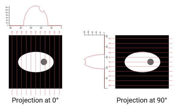
When X-rays go through the object in the 0° direction, we obtain the projection shown on the left. The gray “yolk” causes a dent in the projection due to its lower density than the surroundings. At 90°, as shown on the right, the dent appears in the center.
We can convert these projections into gray-level images and add them, as shown below. The “dent” in each projection indicates where the “yolk” is. We can roughly figure out where the “yolk” is by adding two projections.
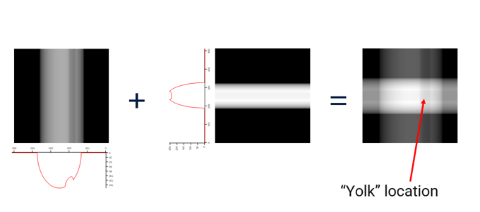
The reconstruction from two projections might not look like much, but you can already see the rough size of the “egg” and the location of the “yolk.”
As you increase the number of projections, the reconstructed cross-section becomes more refined.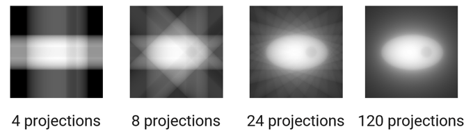
In theory, the number of projections you need, N, to accurately reconstruct the original image is calculated as
N = Field of view / voxel size.
Remember the example of the Algebraic Reconstruction Technique? The field of view was two pixels wide. So N = 2. We used 0 and 90°, two projections, to solve four relational equations. That is the exact amount of information we need to reconstruct the original image.
You might have noticed the images above look blurred. Now, let’s consider why they are blurred. To understand what blurs the reconstructed image, we must go back to the math behind it.
We will skip the derivation of the relationship, but the 1D Fourier transform of the projection p(t, θ) is equal to a slice, at θ, of F(u, v) that is a 2D Fourier transform of µ(x, y). These relationships are visually summarized below.
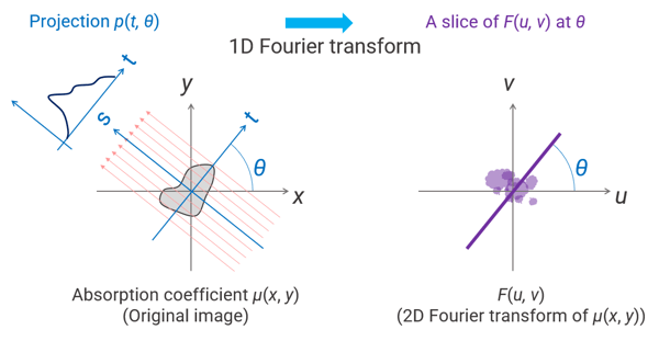
This set of relationships is called the Fourier slice theorem or the projection slice theorem. It is a convenient theory, as we will see next.
The Fourier slice theorem tells us all we need to do to reconstruct the original image is as follows:
- Collect projections.
- Fourier transform projections.
- Add all projections in Fourier space.
- Inverse Fourier transform the results.
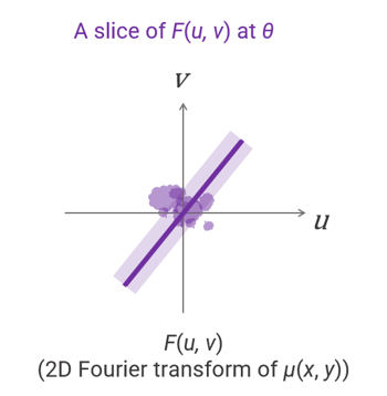
These are pretty straightforward steps to follow. However, we need to consider that a “slice” of F(u, v) is not a line, as shown in the figure above, but a rectangular shape with a width, as shown below.
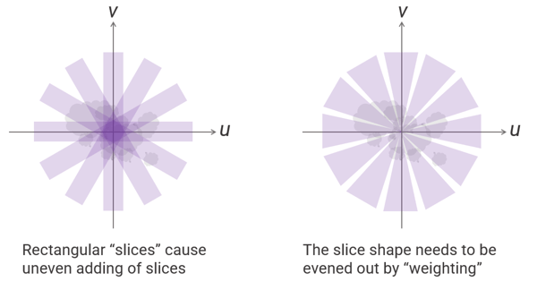
This width causes uneven adding, as shown below on the left. The center area has many data points added due to the overlapping rectangular “slices,” while the edge has fewer data points due to the gaps between “slices.” This is what causes the blurring of the reconstructed image we saw before. To avoid this issue, we need to downweigh the center part of the slices, as shown on the right.
This downweighing process is called filtering. Typical filters include the ramp, Hann, Ramachandran-Lakshminarayanan, and Shepp-Logan filters.
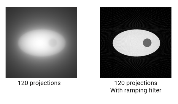
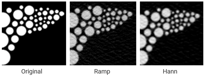
The blurriness in the cross-section of the “egg” reconstructed using 120 projections disappears after applying the ramping filter, as shown below.
The graph below shows the shape of different filters.
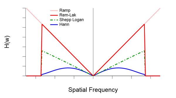
All filters work well, but they produce slightly different results. Examples of the ramp and Hann filters are shown below. The ramp filter adds noise but preserves the edges well, while the Hann filter adds less noise but blurs the edges.
There you have it. This is how CT images are reconstructed using the FBP algorithm. As mentioned earlier, the calculation gets more complicated for cone beam geometry, but the core concept is the same.
Further Reading
If you want to learn more about reconstruction and other theories used in X-ray CT, I’d recommend “X-ray CT: Hardware and Software Techniques” by Toda, H.
If you are interested in how the Fourier slice theorem is derived but are not a big fan of reading textbooks, you can watch this video: Intro to Digital Image Processing by Rich Radke - # 18 Reconstruction from parallel projections and the Radon transform.
We only mentioned it briefly here, but a Fourier transform is an important concept and appears everywhere in physics. If you want to understand what it is exactly and why it’s so widely used, this visual representation of the concept might help: But what is the Fourier Transform? A visual introduction by 3Blue1Brown.
Try hands-on exercises
I hope this article helped you understand how CT reconstruction works. But sometimes, it is best to experiment with the technique to truly understand it.
All the source images you saw in this article are available to download. You can use the open-source image processing program ImageJ to run the calculations demonstrated here. All the sample data, tutorial video, and an e-book are available on the on-demand workshop recording page.
If you have any questions or need help finding resources about CT reconstruction, our team of CT experts can help you. You can talk to one of our CT experts by clicking the “Talk to an expert” button at the top right of the page or send us a message at imaging@rigaku.com.