How to Choose kV and Filter for Your Micro-CT Experiment

People often ask me, “What kV and filter combination should I use to collect X-ray CT (computed tomography) data for my sample?” I understand why people ask this; it’s one of the first things I consider when collecting CT data. kV is the voltage to apply to the X-ray source, and filters shift the X-ray energy. Together, the right choice of kV and filter can make the difference between great and bad CT data.

The good news is that you can use some basic guidelines and tools to determine the right combination. In this article, I share an approach to selecting the right combination based on my experiences in our CT applications laboratory. Hopefully, you will find some tips to take away and apply when you plan your next X-ray CT experiments.

1. Why is kV and filter choice important?
2. Know your sample and plan your experiment
3. Consider important data properties before starting
4. Run short test scans and choose the right setting
5. What if my scanner is not capable of running a good scan for my sample?

Why is kV and filter choice important?

Why is it so important? As we discussed in our introduction webinar, X-ray CT is an X-ray absorption imaging technique, and the degree to which a sample absorbs X-rays depends both on the incident X-ray energy and the sample density and thickness.

If the X-ray energy is too high for a given sample density and thickness combination, the sample doesn’t absorb the X-rays enough and you can’t achieve good contrast. If the X-ray energy is too low, X-rays are “hardened” by the sample and the CT image suffers beam-hardening artifacts. This means that “tuning” the X-ray energy to match the sample properties is important for obtaining good CT data, and we do this by changing kV and filters. This is why they are so important.

Let’s look at how kV and filters affect the X-ray energy.

Most laboratory X-ray systems use cone beam geometry and a tungsten X-ray source. These systems generate a polychromatic X-ray beam consisting of X-rays of varying energies or wavelengths. The exact X-ray energy spectrum depends on the applied voltage (kV). Increasing kV increases the average and peak X-ray energies. 

Once you fix the kV value, you can further “tune” the X-ray energy distribution by placing a metal foil between the X-ray source and the sample. The metal foil absorbs or filters out X-rays of a given energy range, depending on the chemical composition and the thickness of the metal foil. This is why they are commonly called X-ray filters.

Below is a plot of X-ray transmission rate vs. energy with different filters, illustrating their effects.

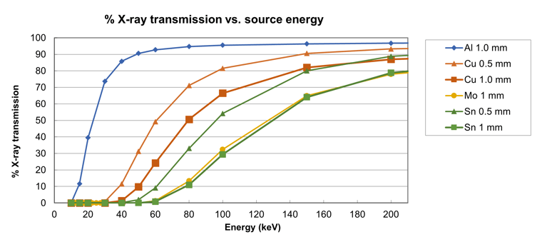
X-ray energy transmission rate dependence on X-ray filters. X-ray attenuation is calculated using MuCalc (Hanna, R.D., Ketcham, R.A., 2017, Chemie der Erde Geochemistry, 77 (4):547.).

The plot above illustrates how an X-ray filter eliminates (filters out) low-energy X-rays from the incident beam, which effectively ‘hardens’ X-rays by shifting the average X-ray energy to higher keV. If beam hardening happens in the sample, that causes artifacts in the CT image. By pre-hardening the X-rays before they hit the sample, you can reduce the beam hardening artifacts.

In the plot above, notice that both the filter material and the filter thickness affect the percentage of transmitted X-rays, and that ultimately affects the effective energy of the filtered X-rays the sample absorbs.

Let’s imagine that you have a sample with higher density, meaning it contains elements with a high atomic number Z, such as iron, or it is very thick—tens of millimeters thick, for example. For this situation, you want to filter out low-energy X-rays to minimize beam hardening. In that case, a 1.0 mm Cu filter would be a better choice than a 1.0 mm Al filter. Depending on the exact density and thickness of the sample, you might even need a Sn filter.

On the other hand, if the sample is made of light, low-density materials, and is small or thin, you want to use low-energy X-rays. In this case, you decrease the kV and use a light and thin filter, such as Al, or eliminate the filter.

To summarize, the combination of kV and filter determines the energy of X-rays the sample absorbs to generate the CT image. The X-ray energy needs to match the sample properly to obtain good contrast and minimize artifacts.

Know your sample and plan your experiment

To tune the X-ray energy correctly, we need to know what the sample is made of and how thick it is.

You don’t need to know the exact chemical formula, but you will need to know the general composition of your sample or approximate density. For example, is it a lightweight foam, an organic material, a rock, an electronic component, or a sample containing heavy metals? The first three are low density, while the others can be high density. It also helps to know your sample size and whether you expect a large void content, as this reduces the total thickness of the material and thus affects the X-ray absorption rate. 

With sample composition and thickness information, you can use some general guidelines to choose your starting point for the kV and filter.

Experimental results in publications are valuable places to look for guidance, as these can provide example combinations of the kV, filter, and sample properties, along with representative images. I recommend you search for CT publications for your sample type.

For example, suppose that you are working with fossilized materials. A quick Google Scholar search of “microct fossils” found 11,800 results. To shorten the list, you can filter out some of the results by making your search criteria more specific to your samples. Although  publications don’t always include data collection parameters, many do.

I’ve listed a few from my search below, with some notes.

• Fossilized shark tooth in rock matrix (~20 mm), 180 kV, Cu filter, voxel= 9 µm (Abel, R., Laurini, C., Richter, M., 2012. Palaeont. Electr 15 (2):6T.)
• Fossils preserved in amber (6 mm), 60 kV, no filter, voxel = 2.7 µm (Dierick, M., et al., 2007. Nucl. Instrum. Methods Phys. Res. A, 580:641.)
• Herpetology fossils review article, 92 ± 40 kV for biological samples, 126 ± 53 kV for fossilized rock samples, filters included none for biological samples, 0.25 – 1.5 mm Al and 0.1 mm Cu for higher density samples (Broeckhoven, C., Plessis, A. du, 2018. Amphib-reptil. 39:377.)
• 3D preserved bat skull, (18.29 mm), 50 kV, voxel = 8.93 µm (Hand, S.J., et al., 2023. Curr. Biol. 33:4624.e21.)
• Bones from extant and extinct archosaurs, 50 kV, no filter; 60 kV, 1.5 mm Al filter, 115 kV, 0.25 mm Cu filter; voxel sizes range from 16 – 78 µm (Anné, J., et al., 2015. PeerJ 3:e1130.)

From this list, you can see that about 120 kV with a Cu filter would be a good starting point for fossils in rock form, while 50-60 kV with Al or no filter would work better for bones and amber. Now, you have a starting point, and all you have to do is test a few scan conditions to fine-tune them.

When querying your results, I recommend that you note the X-ray power, field of view (FOV), voxel size, spatial resolution, scan time, and other parameters that researchers used, as these are also very useful reference points.

For quick reference, I have included a table below with recommendations based on published examples and my personal experience collecting CT data (du Plessis, A. et al. 2017, GigaScience., 6:1., Kozatsas, J. et al. 2018 J. Archaeol. Sci. 100:102., Van Offenwert, S., et al. 2021. Sci Data 8,:18., Keklikoglou, K. et al. 2021. J. Imaging, 7(9), 172).

Consider important data properties before starting

Once you have a general idea of what conditions are appropriate for your samples, you might think the next logical step is to collect some CT test scans. However, I recommend you first ask yourself what metric(s) you will use to assess or score CT data for each test condition before you start collecting scans. Good planning at this point will save you time later.

Those metrics may vary depending on the ultimate goal of your CT experiment. Signal-to-noise ratio (SNR) and contrast-to-noise ratio (CNR) values are commonly used as image quality metrics; however, there are different ways to evaluate the image quality and different metrics you might want to consider (Kalendar, W.A., Computed Tomography: Fundamentals, System Technology, Image Quality, Applications, 3rd Edition | Wiley” 2017.  Nardelli, V.C., et al., 2012. Meas. Sci. Technol. 23, 105006., M., le Roux, S.G., et al., 2020. Mater. Today Commun. 22:100792., Zwanenburg, E.A. et al., 2023. Compos. B. Eng. 258, 110707., Rodríguez-Sánchez, Á., et al., 2020. Precis. Eng. 66:382.).

For example, you may want to perform quantitative analyses of various phases of materials in your CT data. Before you can do that, you will need to segment the CT data into multiple phases. In that case, your criteria would be how well peaks representing these phases in the histogram are separated. For example, you might ask how easily you can segment these phases by simple gray-level thresholding.

How well these peaks are separated depends on SNR and CNR. However, looking at SNR and CNR alone does not tell how well these peaks are separated. Evaluating the peak separation using a histogram is a more accurate and appropriate way to assess the data quality.

Another metric is the level of artifacts. The presence of artifacts can also affect data quality. It makes segmentation more difficult and obscures important regions of interest. For example, if you are performing failure analysis for a part or component, you may only be interested in visually inspecting the data to identify failure points. In that case, artifact reduction or correction may be significant because the artifacts can conceal areas of interest in your sample.

No single metric will gauge data quality for every sample type, so it’s important to consider what benchmarks you will use to compare your CT data.

Run short test scans and choose the right setting

Now, you have the starting conditions you extracted from publications or general guidelines and an idea of how you will assess image quality for each setting. You’re ready to collect some data. Collect some short test scans for your sample and evaluate them based on the criteria you chose above. You should also perform a quick analysis at this point to ensure that you can segment phases, see the features you are looking for, or measure specific dimensions before you commit to running longer, possibly overnight, scans.

Let’s look at tests performed for two examples: polymer and metal samples with small voids. Remember that sample density will also affect our data collection parameters, so I chose these examples to illustrate how settings can change depending on density. We will also vary the size of the polymer sample to see how scan conditions might change with size.

For both test cases, we will evaluate simulated CT data calculated using the program NoviSim. To see the isolated effects of kV, sample density, and sample size, we will keep the X-ray power fixed for all X-ray CT simulation experiments because the X-ray focus size is affected by the total X-ray power, and we want to keep the focus size the same for a fair comparison. The filter will also remain the same.

Polymer sample example

Our first test case will explore the ideal kV setting for a porous low-density polyethylene (LDPE) polymer sample. We will also examine how your kV choice may change depending on sample size. We start with a quick search of the literature to see how others collected data for similar samples. A quick Google Scholar search of “microct LDPE additive manufacturing” resulted in 453 results, and a review of a few of these publications indicates that the range of kV used was 20 kV – 55 kV. Also, many of the representative samples were small (<10 mm) in these publications. No filter was generally mentioned in publications, but we can reasonably guess that no filter was used at these low energies. (Pérez-Tamarit, S., et al., 2018. Eur. Polym. J. 109:169. Peng, F., et al., 2019. ACS Appl. Polym. Mater. 1: 275. Karimipour-Fard, P., et al., 2021. J. Cell. Plast. 57, 623–642.)

Let’s start by looking at simulated data for a 1 mm diameter cylinder of a porous LDPE sample. CT data were calculated using 20 kV and 50 kV. For this exercise, we assume that an important data property is the ability to easily segment LDPE from the air or voids .

A quick visual inspection of a 2D slice from each scan below shows that data collected at 20 kV have worse cupping artifacts than that collected at 50 kV. You might think this means the 50 kV data is better, but that is not necessarily the case. The contrast between LDPE and air and the SNRs affect how easily we can segment these two phases. So, the presence of cupping artifacts alone does not conclude that the 20 kV data is bad.

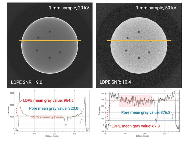
Simulated CT cross sections and gray value plots of data at 20 kV and 50 kV (sample: 1 mm LDPE)

Let’s look at the gray values. The figure above also shows gray level plots along the yellow lines in the cross-sections. These plots show different LDPE mean gray levels for 20 and 50 kV. The LDPE average gray level is ~965 for 20 kV data and ~376 for 50 kV data, indicating there is greater absorption at lower kV. If we look at the SNR for LDPE in each, the values are 19.0 and 10.4 for 20 kV and 50 kV, respectively. Taking these two observations together, thissuggest that 20 kV is a better choice for this sample. 

Let’s take a look at what happens when we perform segmentation. The figure below shows segmentation results using Otsu binarization, where LDPE polymer is labeled blue and voids are labeled red. Throughout the 50 kV image, some voxels are mislabeled as air/void (red), while this is not the case for the 20 kV image. This happens because the gray level of some void voxels is high enough to occur within the LDPE peak of the above histogram. As a result, Otsu binarization for 50 kV data incorrectly assigns some LDPE voxels as void. This strengthens the reasoning that 20 kV is better than 50 kV for this 1 mm LDPE sample.

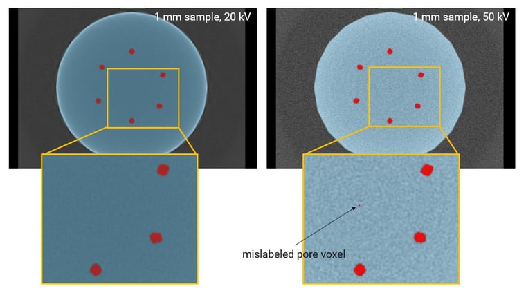
Simulated CT cross sections and gray value plots of data at 20 kV and 50 kV (sample: 1 mm DLPE), segmented into LDPE (blue) and voids (red) by Otsu binarization.

We can take this example further and ask whether 20 kV remains suitable for larger diameter polymer samples. To test this, we will examine CT data simulated for a 40 mm LDPE cylinder collected with no filter at 20 kV and 50 kV.

As shown below, the gray value plots along the yellow lines show that the 20 kV data is much noisier than 50 kV. Specifically, there is greater variation in intensity in the 2D plot for 20 kV data, illustrated by the thicker shaded area, compared to 50 kV. This difference in the noise level can be quantitatively evaluated by calculating SNRs. The 20 kV and 50 kV data’s SNRs are 4.19 and 6.57, indicating that the 20 kV data has a higher noise level, which tends to make image segmentation difficult.

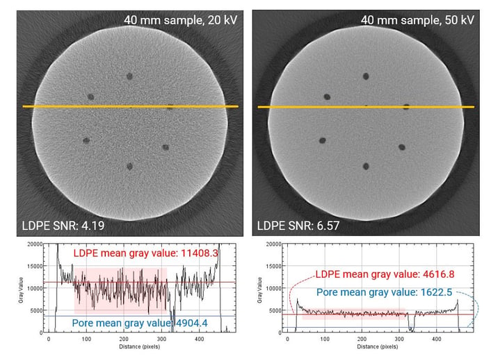
Simulated CT cross sections and gray value plots of data at 20 kV and 50 kV (sample: 40 mm DLPE)

The figure below shows the results of Otsu binarization. As expected from the high-level noise or low SNR, the 20 kV data shows many LDPE (blue) voxels mislabeled as void (red).

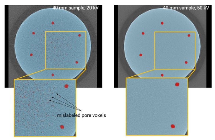
Simulated CT cross sections and gray value plots of data at 20 kV and 50 kV (sample: 40 mm DLPE), segmented into LDPE (blue) and voids (red) by Otsu binarization

These results illustrate that the choice of kV for a given material will vary depending on the size and thickness of the sample. Specifically, 20 kV seems best for small samples of LDPE and 50 kV is more suited for the larger LDPE sample with a 40 mm diameter.

These results also demonstrate that segmenting the test scans can be an important step when evaluating CT data quality. Simply judging which scan is better based on the contrast or artifacts can lead to a wrong conclusion.

Metal part example

For this example, we’ll use a metal part to examine the effects of different types of metals in kV and filter choice. Because metals have high density, CT data for metals are prone to beam hardening artifacts. We’ll use higher kV and introduce an X-ray filter to reduce the artifacts.

What should be the important data property for metal parts? When investigating machined parts, it’s common to investigate part dimensions, conduct geometric dimensioning and tolerancing (GD&T) analysis, or compare the CT scan with the CAD (computer-aided design) file for the actual versus nominal comparison. These dimensional analyses require surface determination, a step where the hard surface of an object is defined to allow mechanical dimensional analysis. In this case, the ease and accuracy of surface determination would be an important factor.

For 3D-printed parts, porosity, cracks, and other analyses like surface roughness might be of interest, and the absolute dimensions are often less important. In this case, elimination of artifacts and sufficient spatial resolution might be as important as surface determination.

For this exercise, data were simulated for a small metal motor at different kV and filter combinations. Simulations were calculated for Al, Ti, and Fe parts with 0.5 . The figure below shows simulations at 100 kV for these three parts with 0.5 µm Al filter.

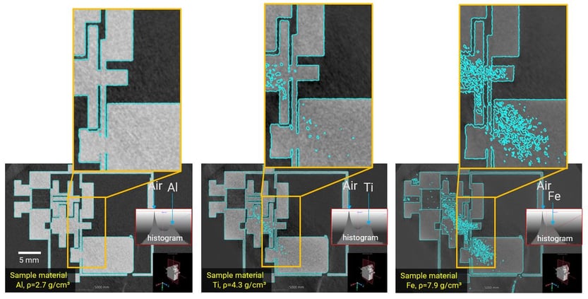
Simulated CT data for Al, Ti, and Fe parts at 100 kV with 0.5 µm Al filter. Surface determination was applied using VGSTUDIO MAX.

Data for the Al sample calculated for 100 kV with 0.5 µm Al filter, shows successful surface determination, whereas Ti and Fe with greater density have significant artifacts that hinder surface determination. The histogram for Al shows good separation for the air and Al, making the surface determination successful. Meanwhile, the air and the metal peaks become closer as the sample density increases for Ti and Fe, making surface determination more difficult. This means samples containing Ti or heavier metals will require higher energy to reduce artifacts.

CT data were also simulated for the Ti sample at 100 kV, 150 kV, and 200 kV coupled with a Sn 0.5 µm filter to see the effect of increased kVs and a more absorbing filter. The resulting cross-sections are shown below, with surface determinations and histograms from which each of the surface determinations were made.

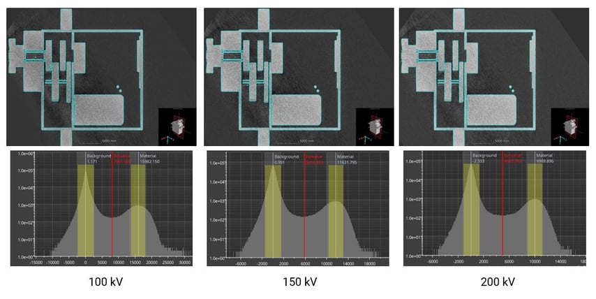
Simulated CT data for Ti at 100, 150, and 200 kV with 0.5 µm Sn filter

Using VGSTUDIO, the background (air) and material (Ti) peaks were automatically selected and highlighted in yellow in the histograms above. The automatically determined isovalue is depicted by the red line. All histograms show good separation between the air and Ti peaks, so you might expect the surface, which is the border between the air and Ti, can be easily and accurately determined. However, there are subtle differences among these three scans.

The surface determination results for small gears are shown in the figure below. They all show “voids” falsely identified inside of the solid Ti parts. Also, some of the gear teeth seem deformed. However, the amount of these false voids and deformation decreases as the used voltage increases, and the 200 kV data resulted in the best surface determination. 

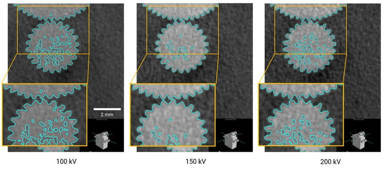
Surface determination results for data simulated for a Ti part at 100 kV, 150 kV, and 200 kV.

There are tools within software like VGSTUDIO MAX to get rid of false voids. However, the deformation of the gear teeth is harder to correct by software tools. Therefore, we can conclude that the 200 kV with 0.5 µm Sn filter is a better choice for this Ti part.

These examples demonstrate the general need for higher voltage and more absorbing filters for metal parts. They also illustrate that the types of metals can affect the best kV and filter combination even when the object size and shape are the same.

So, what’s the takeaway from these two examples? The first example tells us that 20 kV with no filter is a good place to start for small (~ 1 mm) polymer samples, but a higher kV is required as the sample size increases.

The second example tells us you can use 100 – 200 kV with an Al filter for light metals. For most transition metals, a higher kV and more absorbing filter, such as Sn, works better. In the previous example, 200 kV provides the best surface determination among the simulated data. And, of course, the best kV and filter combination will also depend upon the thickness of your metal sample, as we observed in the case of the LDPE sample.

Once you’ve settled on a choice of kV and filter, you might still consider running longer test scans and repeat segmentation and/or additional analyses to ensure that you also optimize for the best signal-to-noise ratio.

What if my scanner is not capable of running a good scan for my sample?

When performing your tests, you may find that your X-ray CT scanner can’t collect the right data for your sample. There can be many reasons why that might happen. For example, your X-ray CT system may have kV limitations, sample size limitations, or other restrictions. You can sometimes overcome the sample size limitations by cutting the sample. In other cases, the constraints of your X-ray CT system may require you to consider other data collection options.

For example, you can explore contract service laboratories or X-ray CT vendors. Some university imaging facilities offer data collection for a fee. Additionally, some X-ray CT vendors provide data collection services for a fee or to demonstrate instrument capabilities. In rare cases, you might need advanced imaging capabilities for your sample or project, such as monochromatic, parallel, or extremely bright X-rays. Then, you might consider data collection using a synchrotron. Data collection at these facilities generally requires a proposal to define scientific merit and experimental requirements. Here are a few examples of facilities equipped with CT scanners:

• The University of Delaware Advanced Materials Characterization Lab
  https://amcl.udel.edu/
• The University of Texas High-Resolution X-ray Computed Tomography Facility
  https://www.ctlab.geo.utexas.edu/
• Applied Technical Services, LLC
  https://atslab.com/

Takeaways

I hope you find some of the information in this article useful as you navigate CT data collection. If you still feel unsure where to start, feel free to reach out to one of our CT experts by clicking the ‘Talk to an expert” button at the top right of the page or send us a message at imaging@rigaku.com. Finally, let us know if you have tips or find great tools that would help others improve their CT data collection and analysis capabilities.